
With reading week over, this week began with a one to one review of what my programme of study entailed. One thing that did not occur to me was the fact that my research topic seems to be something that will be undertaken on a solo basis. I had assumed that I would try and ‘shoehorn’ in my topic with a team of others, although the way in which this would happen was vague at best. In hindsight, I think this is the best option as it leaves me to decide how best to tackle the subject on my own terms and in a way that would suit the visualisation of audio. My only other concern about this was the fact that I may not have as long a showreel at the end of the course if I was working on my own. However, this seems to be a trivial point as the longest films of last year were indeed from two individual students. Additionally, I can, and may very well, be asked to contribute the odd shot to other teams work depending on what they need to enhance their work, as indeed may I! So, the next step for me is to start thinking about how I will translate the idea into a narrative or story that can be broken down into its constituent parts before planning on the project can proceed.
Today, Monday the 21st October, also saw the remainder of the initial stage of the NURBS assignment completed. I have completed the radiator, guitar cables and wall picture in addition to other details I added over the weekend. The next stage will be doing an Ambient Occlusion pass for a basic render. If I have time, I wil texture the scene, but before that I will focus on starting the polygonal modelling assignment.

And the first Ambient Oclusion Pass (combined with a light source):

The remainder of the week focussed on getting through the rest of the dynamics lessons on digital tutors. starting the polygonal modelling assignment and continuing with my research into visualising sound.
- Per Particle Expressions – You may have a scene were you don’t need your particles to last forever, as this is wasteful! So, we can use per particle expressions to control when the life of the particle will end and how it will do so. Select the particles and go to the nPartcle Shape tab to access the attributes. (Per Particle Array) Lifespan PP – right click to open the expression editor, use the runtime expression afdter dynamics button and type in the code as seen in the example below:
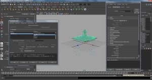
Once it is opened, you copy and paste the expression in the ‘select object and attribute’ box, then add ‘= 0’ to the end of it. Click Create – now, however, they die off right away, so we need to change the expression so that they die off once they reached around -10 on the Y axis. We can do this by adding in the following code before the last expression:

vector $ppos = nParticleShape1.position;
if ($ppos.y < -10) nParticle Shape1.lifespanPP=0;
So, what we’re saying here is if we assign the position of the particle mposition to a variable ppos, then we can use an ‘if’ statement to tell it to die off once it has reached the -10 point of the Y axis. Otherwise it will be displayed.
- Per Point Emission Rates – this example showed me how to use specific points on a mesh that would only act as emitters for the particles, rather than the whole thing. After reducing the emitter rate and making the plate and fries in the scene passive colliders, I selected the emitter/nParticles menu/Per Point Emission Rates – then selected the ‘Use Rate PP’ attribute in the channel box. The reason being once I selected the mesh, all of the emitter shapes are made available in the channel box.
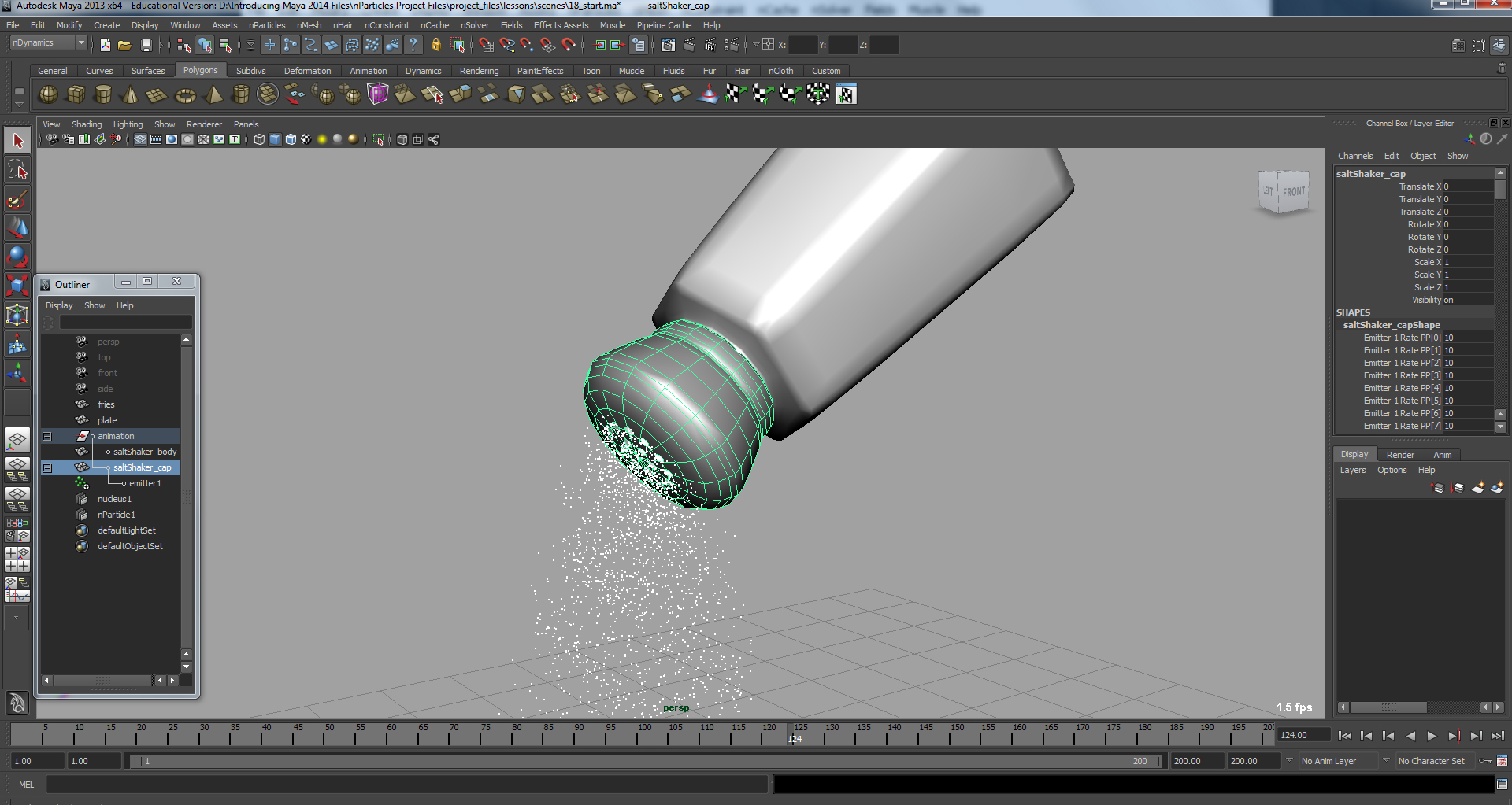
Now I selected the vertices where I wanted the particles to come from, i.e. the shaker holes only, and the highlighted vertices would be shown in the status bar at the bottom of the screen as a range when I typed in ‘ls -sl’ into the MEL command line. In this case something like [0:428] with the odd vert I had left on its own. So, now I had to select all other vertices and make the emission rate 0. To tidy up the animation I set the stickiness attribute to 2 for the salt particles to stick to the fries and plate.
- nParticle Liquid Simulation – (Jam on bread) this lesson involved using the water preset for the nPartcle tool and using the option box to allow sketching on to the surface of the mesh directly (Select the mesh and ‘make live’ first of all). NB – one problem I had was that I could not draw on the surface of the mesh, only where the vertices where placed. I must solve this issue later! Anyway, I managed to work around it with the following basic settings: no of particles 10; max radius 0.5; make them a purple shade in colour! So, make the mesh ‘not live’, lower it and make it a passive collider. Go to the particles liquid simulation properties and up the viscosity to around 10 to make it thicker. Select the bread mesh and set the friction to 0.8 (collision attribute), while the stickiness is 1 so it will stack up. As for the particles, the liquid radius scale determines how much overlapping there is, leave it at 1 for now. NB – An interesting point to note was that by animating this scale, an organic kind of ‘heaving’ look can be achieved! Additionally, the rest density defines how many particles can stay on top of one another, while the incompressibility determines how rigid a substance is – the higher the value the more rigid, but too high and it can explode! Leave it at 1 for a liquid type compression.
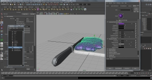
- Once at this stage, it needed to be converted into an output mesh. So, set the jam to be the current state, once you have the simulation presentable, make the knife a passive collider, and adjust the animation of the knife to suit as it may not be spreading the jam appropriately. To do this, open the graph editor and change the Y translation so it intersects the jam. You can also change the attibutes of the knife: stickiness 1.5; friction 1.0; Now, convert nParticles to Polygons (modify menu). At first it disappears because we need to raise the blobby radius in the output mesh attributes to see them. Other attributes to tweak include the Threshold and the Mesh Triangle size, which is important, as the smaller the size the better the detail on the mesh. To be honest, it didn’t look that impressive, but I don’t know how much of that depended on my tweaking of the values. I continued nonetherless!
- It’s also possible to change the mesh methods to Terahedra, Acute tetrahedra or quad mesh (not adivisable!). Then, assign a material (if you happen to deselect the mesh you can go to nSolver menu – AE display – check the material nodes option – now you have access to the material in the attributes!)
- Finally, playblast the animation!

- Emitting Bolobby Liquid nParticles – this example involves pouring sauce from a bottle onto a steak using a surface emitter parented to the bottle. Using water as the emitter type, set the particle size to around 0.5 and up the rate to around 1000. It’s useful to note that you can reshape the surface emitter (in this case a planar surface from a circle) and the resultant shape will change the flow of particles.
The problem now is that it’s too intense, like a waterfall! We need to go to the nucleus tab, scale attributes, so that we can set the scene scale. The plate is around 30cm (0.3m) so in space scale = 0.3/6 (this is the number of grid units) = 0.05
We also need to fake some internal resistance (Damp) to the particles to make them seem thicker. (In dynamic properties for nParticleShape) Around 0.4 seems appropriate. Make the plate and the steak passive colliders. The ‘slices’ that appear in the particles here are caused by gravity – to make it more blobby, go to nucleus tab and change the quality solver attribute: substeps 6; max collision iterations 8.
Now to adjust the friction settings of the steak! Collisions – solver display – collision thickness. For a porous material like steak, you want the particles to sink into it a bit (they float at the moment). They need a negative value in the thickness attribute, e.g. -0.025. Also, try: friction 0.5; stickiness 0.2. For the particles, liquid simulation attribute – viscosity 3.00 (which makes it thicker); shading – change the colour for reasons of aesthetic!
So far so good. However, the particles are too small. I fwe increase the radius it messes the whole simulation up. So, the answer here is to cache the simulation. To do this – select the particles, nCache menu – create new cache. Play the simulation and hit escape when you have sufficient frames – in this case, around 70 frames in. Now reset the timeline to 70 frames so you’re only dealing with the relevant frames. With the simulation cached, you can scrub through it with no latency issues. In addition, you can also change certain attributes, inlcuding the radius!
So, once that has been accomplished, you can now asign a new material. In this case a Blinn with reduced eccentricity, increased specular colour and specular roll off. After all of this it still looks a bit blobby though! We can sort this ot by going to the radius scale ramp (nParticleShape attribute) and using the radius scale to change the size from where it comes out of the neck to where it hits the steak. Change the Radius Scale Input to ‘Age’. So we’ll start with a bigger size and ramp it down to a smaller one. The settings were around 0.25 for the bigger, with the smaller one being ‘eyeballed’.

Now in the Shading attribute, set Threshold to around 2.0 – you may get clipping in the viewport but when rendered it may not appear. Now, to render the whole thing we need to batch render. Go to render settings, set Frame/Animation Ext to ‘name.(hash key).ext – set start and end frames to the cached version (70) – in the MEL command line, type in BatchRender and press enter.
- Thick Cloud nParticles – the last lesson in this set is dedicated to creating smoke coming out of a chimney stack. Create a thick cloud emitter (rendered with a fluid texture). There are a number of other presets to choose from within the npThickCloudFluid tab. It’s better here to have fewer particles as the particles are dense and have a fair amount of detail already. Now move the emitter to the mouth of the stack.
- the emitter attributes: basic emitter attribute – rate around 5.00; Emitter type – directional.
- nPartcleShape – particle size radius around 1.00.
- set the distance/direction attribute to Direction Y = 1 (so it goes up!) and spread to 0.2
- Basic emission speed to around 4.0
- At this stage it loooks a little too solid! We can alter this by going to the nParticleShape shader/opacity scale and using ramp value as seen below to complete the effect.

Overall, these lessons have been basic but a useful way into particles and some of the possibilities they offer. I will attempt to use some of what I have learned for initial tests at this early stage of my research to see if there is room for further development.
Thursday 24th October
It is also worth noting this week, that we had 2 guest lecturers in the shape of Kieran Baxter and Chris Rowland. Kieran has been a masters student here whom is now doing his phd in the field of photogrammetry through aerial photography of heritage sites. His work is very impressive and he suggested using Photoscan as a useful piece of software to tie images together for this kind of work. His website is topofly.com.
In a vaguely related vein, Chris has been diving and surveying ship wrecks and oil rigs with sonar and new blue lazer technologies to create accurate data sets and visualisations of stricken or wrecked vessels, which until recently have only yielded poor results for salvage companies or other interested stakeholders that deal with disaster type scenarios. His work is also focussing on offshore renewables and the potential dangers for the public and sealife. The key thing to remember from both of the speakers today was that they generally work through a process of:
Reflection – Planning – Acting – Observing – Reflection….(as a loop – where each iteration is a separate case study that yields its own conclusions or data sets).
Friday 25th October
Jin’s class today was looking at texturing in Maya. Focussing on the ‘shoe’ project for polygonal modelling, we looked at techniques using projections in Maya to begin with. Basic shapes are suitable for projections but when it comes to more complex organis shapes, UV mapping is the way to go. However, rather than delving into how to do it in Maya, Jen suggested we use what the Industry Professionals use – UVLayout.com – this site has software that will simplify the process of unwrapping the uv’s into suitable shapes for mapping. As yet I have not had the opportunity to use it, it’s a fee paying piece of software, hopefully the university will provide! So, this has yet to be resolved.
In addition, some useful techniques in Photoshop were discussed: the use of the clone stamp or healing brush tool are useful for painting in/out shadows or highlights or extending a texture so that the uv’s are completely covered. Layer blending modes are very useful as well obviously – the use of the screen blending mode allows the snapshot of the uv’s imported from Maya to be ‘see through’ to the layer below, making it easier to work on where the textures are to be placed etc. The stitch tool can be very useful for the creation of a larger texture from several photographs taken at slightly different angles.
Jin aso looked at a couple of similar techniques in Nuke, which I have yet to attempt. I plan to do some introductory lessons in Nuke next week.
